-
Data Structures and Algorithms
- Key topics: arrays, linked lists, stacks/queues, hash tables, trees (binary trees, AVL trees, red-black trees), heaps, graphs, and string operations.
- Common algorithms: sorting (quicksort and merge sort), binary search, DFS/BFS, dynamic programming, greedy algorithms, sliding windows, and two pointers.
- Recommended resources:
- Books: Introduction to Algorithms, 剑指Offer (Coding Interviews).
- Practice platforms: LeetCode (Top 100 problems), Nowcoder (past interview problems from Chinese companies).
- Study tips: practice by topic (such as dynamic programming), and summarize templates and common optimization techniques.
- Problem list by 三叶
- Algorithm templates
- Common Go data structures
-
Computer Networks
- Core concepts: the TCP/IP protocol stack, HTTP/HTTPS, DNS, WebSocket, the TCP three-way handshake/four-way teardown, and congestion control.
- Common questions: HTTP status codes, RESTful API design, cookies versus sessions, and the HTTPS encryption process.
- Recommended resources:
- Books: Computer Networking: A Top-Down Approach.
- Articles: MDN Web Docs and Ruan Yifeng's blog posts on HTTP.
-
Operating Systems
- Core topics: processes/threads, deadlocks, memory management (paging/segmentation), virtual memory, file systems, and I/O models.
- Common questions: thread synchronization (locks and semaphores), interprocess communication (IPC), and context-switch overhead.
- Recommended resources:
- Books: Modern Operating Systems, Operating Systems: Three Easy Pieces.
- Videos: MIT 6.828 (operating systems course).
-
Databases
- SQL: complex queries (JOINs and subqueries), index optimization, ACID transactions, and isolation levels.
- NoSQL: Redis (data structures and persistence) and use cases for MongoDB.
- Common questions: how indexes work (B+ trees), slow-query optimization, and MVCC.
- Recommended resources:
- Books: High Performance MySQL, Redis设计与实现 (Redis Design and Implementation).
- Tools: use EXPLAIN to analyze SQL execution plans.
The following are detailed recommendations and focus areas for backend interviews in Golang/Python/Java/C++:
- Language features
- Concurrency model:
goroutine,channel(buffered/unbuffered),select, and thesyncpackage (Mutex and WaitGroup). - Memory management: escape analysis, tri-color marking in GC, and memory alignment.
- Interfaces and reflection: implicit interface implementation and how the
reflectpackage works.
- Concurrency model:
- Common questions:
deferexecution order and pitfalls (such asdeferand variable capture in closures).- The underlying implementation of
sliceandmap(growth mechanisms and concurrency safety). - Use cases for the
contextpackage (timeouts and cancellation propagation).
- Interview focus:
- Demonstrate an understanding of highly concurrent workloads (such as implementing the producer-consumer model with
channel). - Prepare a concurrent project implemented in Go (such as a distributed task scheduler).
- Demonstrate an understanding of highly concurrent workloads (such as implementing the producer-consumer model with
- Microservice frameworks: Gin (routing and middleware mechanisms) and Echo.
- Ecosystem tools: gRPC (Protocol Buffers) and dependency management with Go Modules.
- Books: Go语言设计与实现 (Go Language Design and Implementation), Go语言高级编程 (Advanced Go Programming).
- Source code: read the standard library source (such as the
net/httpandsyncpackages). - Practice: implement a highly concurrent service in Go (such as a WebSocket chat room).
- Project: Go interview collection
- Project: Go algorithm templates
- Language features
- Dynamic typing:
duck typing,MRO(method resolution order), and theGIL(global interpreter lock). - Advanced syntax: decorators, generators, context managers, and metaclasses.
- Memory management: reference counting, garbage collection, and optimization with
__slots__.
- Dynamic typing:
- Common questions:
- Differences between multithreading and multiprocessing (the impact of the GIL).
- How shallow and deep copies are implemented (the
copymodule). - Coroutines and asynchronous programming (
asyncioandasync/await).
- Interview focus:
- Emphasize development efficiency and scripting skills (such as experience developing automation tools).
- Explain the limitations of the GIL and how to work around them (such as multiprocessing plus a message queue).
- Web frameworks: Django (ORM internals and middleware) and Flask (request contexts and blueprints).
- Data processing: Pandas and NumPy (vectorized operations).
- Books: Fluent Python, Effective Python.
- Study: the official Python documentation (with a focus on CPython implementation details).
- Practice: build a high-throughput API service with an asynchronous framework (such as FastAPI).
- Language features
- JVM: the memory model (heap, stack, and method area), class loading, and GC algorithms (CMS and G1).
- Concurrent programming:
synchronized,volatile,ThreadLocal, andAQS(AbstractQueuedSynchronizer). - Collections framework:
HashMap(red-black tree optimization) andConcurrentHashMap(segmented locking/CAS).
- Common questions:
- Compare the time complexity of
ArrayListandLinkedList. - How dependency injection works in Spring (BeanFactory vs. ApplicationContext).
- Practical JVM tuning (OOM diagnosis and GC log analysis).
- Compare the time complexity of
- Interview focus:
- Explore JVM and framework internals (such as Spring AOP's dynamic proxy implementation).
- Draw on distributed systems experience (such as implementing microservices with Spring Cloud).
- Core syntax: the collections framework (HashMap source code), multithreading (thread pools and CAS), the JVM memory model, and garbage collection algorithms.
- Frameworks and ecosystem: Spring (IoC/AOP), Spring Boot auto-configuration, and how MyBatis works.
- Common questions:
- The HashMap growth mechanism
- How ConcurrentHashMap ensures thread safety
- The Spring Bean lifecycle
- Practical JVM tuning experience
- Recommended resources:
- Books: Effective Java, 深入理解Java虚拟机 (Understanding the JVM).
- Source code: the JDK core libraries and Spring Framework source.
- Mainstream frameworks: Spring Boot (how auto-configuration works) and MyBatis (SQL mapping through dynamic proxies).
- Microservices: Spring Cloud (service registration/discovery and the Hystrix circuit breaker).
- Books: 深入理解Java虚拟机 (Understanding the JVM), Java Concurrency in Practice.
- Source code: the JDK collections framework and Spring core modules (such as
spring-core).
- Language features
- Memory management:
new/deleteversusmalloc/free, and smart pointers (unique_ptrandshared_ptr). - Object-oriented programming: virtual function tables (vtables), multiple-inheritance pitfalls, and RAII.
- Templates and STL: template metaprogramming and container internals (
vectorandmap).
- Memory management:
- Common questions:
- Move semantics (
std::moveand rvalue references). - The role of virtual destructors.
- Uses of the
constkeyword (pointers to constants vs. constant pointers).
- Move semantics (
- Interview focus:
- Highlight memory management and performance optimization skills (such as ways to prevent memory leaks).
- Prepare a low-level project (such as a simple database or networking library).
- Common libraries: Boost (smart pointers and thread pools) and Qt (signals and slots).
- High-performance scenarios: memory pool design and zero-copy techniques.
- Books: Effective C++, C++ Primer.
- Study: C++ standards documentation (new features in C++11/14/17).
- Practice: implement STL containers yourself (such as a simple
vector). - Interview experiences: C/C++ backend development interviews
- Basic designs: URL shorteners, counters, distributed ID generation, and caches (LRU).
- Advanced designs: flash-sale systems, social networks (following/followers), distributed file storage, and message queues (Kafka/RabbitMQ).
- Methodology:
- Clarify requirements (QPS, data volume, and consistency requirements)
- Design core components (database/table sharding, caching strategies, and load balancing)
- Address bottlenecks (hot data, distributed locks, and disaster recovery backups)
- Recommended resources:
- Books: Designing Data-Intensive Applications.
- Courses: Grokking the System Design Interview (in English)
- Practice: refer to open-source projects on GitHub (such as TinyURL).
The three-way handshake ensures that a reliable connection is established. The four-way teardown ensures that no data is lost when disconnecting.
- Characteristics:
- Uniquely identifies each row in a table; duplicate and
NULLvalues are not allowed. - Each table can have only one primary key index.
- Uses a B+Tree structure by default.
- Uniquely identifies each row in a table; duplicate and
- Syntax:
CREATE TABLE users (
    id INT PRIMARY KEY, -- Primary key index
    name VARCHAR(50)
);
- Characteristics:
- Ensures that column values are unique;
NULLvalues are allowed (but only oneNULL). - Multiple unique indexes can be created.
- Commonly used to prevent duplicate data (such as email addresses and phone numbers).
- Ensures that column values are unique;
- Syntax:
CREATE UNIQUE INDEX idx_email ON users(email);
- Characteristics:
- The most basic index type, without a uniqueness constraint.
- Speeds up queries while allowing duplicate values and
NULL.
- Syntax:
CREATE INDEX idx_name ON users(name);
- Characteristics:
- Indexes multiple columns together to support queries with multiple conditions.
- Follows the leftmost-prefix rule (query conditions must include the leftmost column to use the index).
- Syntax:
CREATE INDEX idx_name_age ON users(name, age);
- Example:
-- These queries use the index:
SELECT * FROM users WHERE name = 'Alice';
SELECT * FROM users WHERE name = 'Bob' AND age = 30;

-- This query does not use the index (the leftmost column, name, is missing):
SELECT * FROM users WHERE age = 25;
- Characteristics:
- Used for full-text searches (such as
MATCH ... AGAINSTstatements); supports text fields (CHAR/VARCHAR/TEXT). - Available only with the MyISAM and InnoDB (MySQL 5.6+) engines.
- Used for full-text searches (such as
- Syntax:
CREATE FULLTEXT INDEX idx_content ON articles(content); - Example:
SELECT * FROM articles
WHERE MATCH(content) AGAINST('database' IN NATURAL LANGUAGE MODE);
- Characteristics:
- Indexes the first
Ncharacters of a string to reduce storage space. - Requires a balance between prefix length and selectivity (uniqueness).
- Indexes the first
- Syntax:
CREATE INDEX idx_name_prefix ON users(name(10)); -- First 10 characters
- Characteristics:
- Used for geospatial data types (such as
GEOMETRY,POINT, andPOLYGON). - Supports spatial queries (such as
ST_ContainsandST_Distance). - Available only with the MyISAM engine (InnoDB supports it from MySQL 5.7+).
- Used for geospatial data types (such as
- Syntax:
CREATE SPATIAL INDEX idx_location ON places(coordinates);
- Characteristics:
- Contains all columns required by a query, avoiding a table lookup.
- Significantly improves query performance.
- Example:
-- If the index is (name, age) and the query needs only name and age:
SELECT name, age FROM users WHERE name = 'Alice';
| Index type | InnoDB | MyISAM | MEMORY |
|---|---|---|---|
| B-Tree | ✅ | ✅ | ✅ |
| Full-text index | ✅ (5.6+) | ✅ | ❌ |
| Spatial index | ✅ (5.7+) | ✅ | ❌ |
| Hash index | ❌ | ❌ | ✅ |
- Primary key index: must be defined for a table explicitly or implicitly.
- Frequently queried fields: index columns used in
WHERE,JOIN, andORDER BY. - Avoid excessive indexing: indexes reduce the performance of write operations (INSERT/UPDATE/DELETE).
- Composite index optimization: prefer highly selective columns as the leftmost prefix.
- In-memory operations: most Redis operations can run in memory, where the data is also stored. Compared with traditional disk-file operations, this reduces I/O and improves speed.
- Efficient data structures: Redis has specially designed efficient data structures such as STRING, LIST, and HASH, which improve read and write efficiency.
- Single-threaded execution: this avoids the overhead and CPU cost of context switching. There is also no resource contention, preventing deadlocks.
- I/O multiplexing: Redis monitors multiple sockets through I/O multiplexing and selects the appropriate event handler based on the events on each socket.
How Does Redis Prevent Data Loss After a Power Failure? How Does It Provide High Availability and Avoid Inconsistency?
Redis is an in-memory database by default, with data stored in memory. To prevent data loss caused by power failures or other unexpected events, Redis provides two persistence mechanisms:
- RDB(Redis DataBase):
- How it works: saves Redis data at a particular point in time (a snapshot) to disk in binary form.
- Triggers:
- Manual: use the SAVE or BGSAVE command.
- Automatic: configure Redis to trigger a snapshot when N data entries have been modified within a specified period.
- Advantages: fast recovery from the file, making it suitable for data recovery. Simple configuration.
- Disadvantages: possible data loss. If data changes between two RDB snapshots and has not yet been saved, some data will be lost when a failure occurs.
- AOF(Append Only File):
- How it works: appends all write commands to a file in Redis protocol format.
- Triggers:
- Sync every second: writes buffered data to the AOF file once per second.
- Sync every change: synchronizes each write to the AOF file.
- Sync disabled: writes to the AOF file only when the server shuts down.
- Advantages: high data safety and a low probability of data loss. Supports efficient data appends.
- Disadvantages: the AOF file may become very large, affecting performance. More frequent file synchronization has a greater performance impact.
Recommendations:
- Enable both RDB and AOF: use RDB for fast data recovery and AOF to ensure data is not lost.
- Configure a suitable RDB save policy: set the RDB save interval and trigger conditions according to business requirements.
- Configure a suitable AOF synchronization policy: choose an appropriate AOF sync frequency while ensuring data safety.
- Primary-replica replication:
- How it works: the primary handles writes, replicas handle reads, and the primary synchronizes data to the replicas.
- Advantages: separating reads and writes improves performance. Data redundancy improves availability.
- Disadvantages: manual failover is required if the primary fails.
- Sentinel mode:
- How it works: Sentinel is a Redis monitoring tool that can monitor multiple Redis instances and automatically fail over when the primary fails.
- Advantages: automatic failover improves availability. Supports primary-replica replication configuration.
- Disadvantages: relatively complex configuration.
- Redis Cluster:
- How it works: shards data across multiple nodes, each responsible for a portion of the data.
- Advantages: linear scalability, improved performance, and high availability.
- Disadvantages: complex configuration and high data migration costs.
- Primary-replica replication consistency:
- Partial synchronization: the primary synchronizes data to replicas immediately after writing it.
- Full synchronization: the primary writes data only after receiving ack confirmations from all replicas.
- Sentinel failover: Sentinel selects a replica as the new primary and synchronizes data.
- Redis Cluster data consistency: uses consistent hashing to distribute data. Supports failover and data migration.
Definition: a large number of cached entries expire simultaneously, causing all requests to access the database directly and triggering a surge in database load or even a crash.
Solutions:
- Randomized expiration times: assign different expiration times to cached entries (for example, a base expiration time plus a random offset).
// Example: set expiration to 60 minutes ± a random 10 minutes
int expireTime = 60 * 60 + (int)(Math.random() * 10 * 60);
- No expiration + asynchronous updates:
- Do not set cache expiration; update the cache periodically with a background thread.
- Use a mutex to prevent multiple threads from updating it simultaneously.
- Multilevel caching: combine a local cache (such as Caffeine) with a distributed cache (such as Redis) to reduce the risk of simultaneous invalidation.
- Circuit breaking and graceful degradation: when the database is under excessive load, enable rate limiting or return default values to protect system availability.
Definition: when a hot cached entry expires, a large number of concurrent requests reach the database directly, causing a sudden increase in database load.
Solutions:
- Mutex Lock:
- When the cache expires, use a distributed lock (such as Redis
SETNX) to ensure that only one thread loads the data.
public String getData(String key) {
    String data = cache.get(key);
    if (data == null) {
        if (lock.tryLock()) { // Acquire the distributed lock
            try {
                data = db.load(key); // Query the database
                cache.set(key, data, expireTime);
            } finally {
                lock.unlock();
            }
        } else {
            // Wait for another thread to finish loading
            Thread.sleep(100);
            return cache.get(key);
        }
    }
    return data;
}
- When the cache expires, use a distributed lock (such as Redis
- Logical expiration:
- The cached data never expires, but stores a logical expiration time. When the data is found to be expired, update the cache asynchronously.
- Preload hot data: refresh frequently accessed data in advance to prevent normal expiration.
Definition: requests for nonexistent data (such as invalid IDs) bypass the cache and query the database directly, causing useless queries to accumulate.
Solutions:
- Bloom Filter:
- Add a Bloom filter before the cache layer to quickly determine whether data exists and reject invalid requests.
if (!bloomFilter.mightContain(key)) {
    return null; // Return immediately without querying the cache or database
}
- Cache null values: when a query returns
NULL, cache the null result with a short expiration time (such as 5 minutes).if (data == null) { cache.set(key, "NULL", 5 * 60); // Cache the null value }
- Parameter validation: validate request parameters in the business layer (such as ID ranges and formats).
- Rate limiting and blocklists: rate-limit or block IP addresses or users that frequently access invalid keys.
| Problem | Trigger | Core approach | Typical solutions |
|---|---|---|---|
| Cache avalanche | Many cached entries expire simultaneously | Stagger expiration, multilevel caching, circuit breaking and graceful degradation | Random expiration, multilevel caching, asynchronous updates |
| Cache breakdown | Hot data expires | Mutexes, logical expiration, preloading hot data | Distributed locks, logical expiration times, background update threads |
| Cache penetration | Queries for nonexistent data | Reject invalid requests, cache null values, validate parameters | Bloom filters, null-value caching, request parameter validation |
- Monitoring and alerts: monitor the cache hit rate and database QPS in real time to detect anomalies promptly.
- Combine strategies: mix the approaches above according to the business scenario (such as a Bloom filter + null-value caching + a mutex).
- Load testing: simulate highly concurrent workloads to verify that the solution is effective.
func main() {
    m := make(map[string]int)

    go func() {
        for {
            m["blog"] = 1
        }
    }()

    go func() {
        for {
            fmt.Println(m["blog"])
        }
    }()

    select{} // block-forever trick
}

// fatal error: concurrent map read and map write
func main() {
var syncMap sync.Map
// store a key-value pair
syncMap.Store("blog", "VictoriaMetrics")
// load a value by key "blog"
value, ok := syncMap.Load("blog")
fmt.Println(value, ok)
// delete a key-value pair by key "blog"
syncMap.Delete("blog")
value, ok = syncMap.Load("blog")
fmt.Println(value, ok)
}
// Output:
// VictoriaMetrics true
// <nil> falseThe underlying implementation of channels in Go can be divided into the following key parts:
In the Go runtime, each channel is represented by an hchan struct, defined in runtime/chan.go:
type hchan struct {
    qcount   uint           // Current number of items in the buffer
    dataqsiz uint           // Buffer size (capacity)
    buf      unsafe.Pointer // Pointer to the ring buffer
    elemsize uint16         // Element size
    closed   uint32         // Whether the channel is closed (0: open, 1: closed)
    elemtype *_type         // Element type information (for type checking)
    sendx    uint           // Send index (position in the buffer)
    recvx    uint           // Receive index (position in the buffer)
    recvq    waitq          // Receive wait queue (sudog linked list)
    sendq    waitq          // Send wait queue (sudog linked list)
    lock     mutex          // Mutex that protects the channel's thread safety
}- Buffered channels: data is stored in the circular queue pointed to by
buf, withsendxandrecvxtracking write and read positions. - Unbuffered channels:
bufis empty, and sends and receives copy data directly between goroutines.
- Buffer not full: write data directly to the buffer and update
sendx. - Buffer full:
- Wrap the current goroutine in a
sudogand add it tosendq. - The goroutine enters a waiting state, releases the lock, and causes the scheduler to switch to another goroutine.
- Wrap the current goroutine in a
- Receiver waiting: copy data directly to the receiver and wake the receiving goroutine.
- Buffer not empty: read data from the buffer and update
recvx. - Buffer empty:
- Wrap the current goroutine in a
sudogand add it torecvq. - The goroutine enters a waiting state, releases the lock, and waits to be woken by a sender.
- Wrap the current goroutine in a
- Sender waiting: copy data directly from the sender and wake the sending goroutine.
waitq: a doubly linked list storing waiting goroutines (sudog).sudog: represents a waiting goroutine and contains:- A pointer to the goroutine.
- The channel it is waiting on and the operation type (send/receive).
- The memory address of the data (for direct copying).
- Set the
closedflag to 1. - Wake all goroutines waiting in
sendqandrecvq:- Senders: trigger a panic (sending data to a closed channel).
- Receivers: return the zero value and
false(indicating that the channel is closed).
- Sends and receives must rendezvous synchronously; data is copied directly from sender to receiver without passing through a buffer.
- If the other party is not ready, the current goroutine joins the wait queue.
- Nonblocking check: iterate over all cases to check whether each channel operation can proceed.
- Random selection: if multiple cases are ready, randomly select one to execute (to avoid starvation).
- Waiting mechanism: if no case is ready, add the current goroutine to every channel's wait queue; readiness on any channel triggers a wakeup.
- Direct memory copying: avoids extra copies between the buffer and goroutine stacks.
- Lock granularity: a mutex (
lock) protects thehchanstate, but wait-queue operations briefly release the lock to reduce contention.
-
Create a channel:
ch := make(chan int, 3) // Create a buffered channel with capacity 3
- Allocate an
hchanstruct and initialize the buffer, lock, and queues.
- Allocate an
-
Send data:
ch <- 42
- Acquire the lock → buffer has space → write data → release the lock.
- If the buffer is full, the current goroutine joins
sendqand blocks.
-
Receive data:
val := <-ch
- Acquire the lock → buffer has data → read data → release the lock.
- If the buffer is empty, the current goroutine joins
recvqand blocks.
Go channels use the hchan struct to manage buffers, synchronization locks, and wait queues, enabling efficient communication between goroutines:
- Buffered channels: FIFO operations based on a circular queue.
- Unbuffered channels: direct data transfer between goroutines.
- Synchronization: relies on mutexes and wait queues, working with the scheduler to block and wake goroutines.
- Closing: handled through a flag and by waking all waiting goroutines.
This design ensures channel thread safety and efficiency under concurrency.
func f1() (result int) {
    defer func() {
        result++
    }()
    return 0
}

func f2() (r int) {
     t := 5
     defer func() {
       t = t + 5
     }()
     return t
}

func f3() (r int) {
    defer func(r int) {
          r = r + 5
    }(r)
    return 1
}G represents a Goroutine (coroutine) M represents an OS thread P represents a Processor
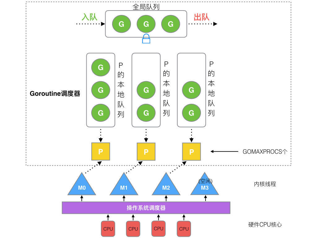
In Go, make and new are built-in memory-allocation functions, but their use cases and underlying behavior differ substantially. The following compares them in detail and explains where memory is allocated:
| Feature | new(T) |
make(T, args...) |
|---|---|---|
| Applicable types | Any type (value types and reference types). | Only the three reference types: slice, map, and channel. |
| Return value | Returns *T (a pointer to type T). |
Returns an initialized value of type T (not a pointer). |
| Initialization | Allocates memory and returns a pointer to the zero value. | Allocates memory and initializes the data structure (such as the underlying array or hash table). |
| Typical use case | Creates a pointer to a value type (such as int or struct). |
Creates an instance of a reference type (such as []int or map[int]bool). |
// Using new
ptr := new(int)    // ptr has type *int and points to 0
s := new([]int)    // s has type *[]int and points to a nil slice

// Using make
slice := make([]int, 10)  // Create a slice of length 10
m := make(map[string]int) // Create an empty map
ch := make(chan int) // Create an unbuffered channelThe Go compiler automatically determines memory allocation through escape analysis, according to the following rules:
- Stack allocation:
- If a variable's lifetime is confined to a function and it does not escape the function, stack allocation is preferred.
- Stack allocation is fast, but space is limited (suitable for small objects or short-lived variables).
- Heap allocation:
- If a variable's lifetime may extend beyond the function (such as when it is referenced by a global variable or returned to the caller), it is allocated on the heap.
- Heap allocation is slow, but offers more space (suitable for large objects or long-lived variables).
-
Allocation behavior of
new:- The pointer returned by
new(T)may be allocated on the stack or heap, depending on whether it escapes.
func foo() *int {
    x := new(int) // x escapes to the heap
    *x = 42
    return x
}
- If the pointer does not escape (it is used only within the function), it may be allocated on the stack:
func bar() {
    x := new(int) // x may be allocated on the stack
    *x = 42
    // x has no external references
}
- The pointer returned by
-
Allocation behavior of
make:- The underlying structures of
slice,map, andchannel(such as a slice's array) are usually allocated on the heap because they need to grow dynamically or be shared across functions.
func createSlice() []int {
    s := make([]int, 100) // The underlying array escapes to the heap
    return s
}
- The underlying structures of
Use go build -gcflags="-m" to inspect whether variables escape:
package main

func main() {
    a := new(int)    // Test new
    *a = 1

    b := make([]int, 10) // Test make
    b[0] = 2
}$ go build -gcflags="-m" main.go
# command-line-arguments
./main.go:4:10: new(int) does not escape # a does not escape and may be allocated on the stack
./main.go:7:13: make([]int, 10) escapes to heap # b's underlying array escapes to the heap| Function | Applicable types | Return value | Initialization | Allocation location |
|---|---|---|---|---|
new |
All types | Pointer | Allocates a zero value | Determined by escape analysis (stack/heap) |
make |
slice, map, channel |
Instance | Initializes the data structure | Usually the heap (underlying structure escapes) |
newreturns a pointer;makereturns an instance.makeis specifically for reference types and ensures the data structure is usable.- The allocation location is determined by escape analysis; underlying structures created by
makeusually escape to the heap.
This problem asks us to write a Go program that prints the numbers 1 to 100 in order in a concurrent environment, while allowing at most 10 goroutines to run simultaneously.
package main

/*
Printing 1 to 100 in order with concurrency in Go

This problem asks us to write a Go program that prints the numbers 1 to 100 in order in a concurrent environment, while allowing at most 10 goroutines to run simultaneously.
*/

import "sync"

// Counter defines a struct that holds the current number and a lock
type Counter struct {
	current int
	mu      sync.Mutex
}

// Define a function to print numbers
func (c *Counter) printNumber(wg *sync.WaitGroup) {
	//defer wg.Done() // Notify the WaitGroup when the function returns
	defer func() {
		if c.current > 100 {
			wg.Done()
		}
	}()

	// Acquire the lock
	c.mu.Lock()
	defer c.mu.Unlock() // Release the lock when the function returns

	// If the current number is at most 100, print it and increment it
	if c.current <= 100 {
		println(c.current)
		c.current++
	}
}

// Define a function to control concurrent printing
func (c *Counter) run() {
	var wg sync.WaitGroup

	wg.Add(10) // Set the WaitGroup counter to 10
	// Create 10 goroutines
	for i := 0; i < 10; i++ {
		go func() {
			for {
				c.printNumber(&wg)   // Call the printing function
				if c.current > 100 { // Exit the loop if the current number exceeds 100
					break
				}
			}
		}()
	}

	wg.Wait() // Wait for all goroutines to finish
}

func main() {
	counter := &Counter{current: 1} // Initialize the Counter struct
	counter.run()                   // Call run to start printing numbers
}
TCP congestion control is a core mechanism for stable and efficient network operation. It prevents network congestion by dynamically adjusting the sending rate. The following explains TCP congestion control step by step:
- Avoid network overload: prevent router or link buffers from overflowing because the sender transmits too quickly.
- Fairness: ensure that connections compete fairly when sharing bandwidth.
- Efficiency: maximize network throughput and minimize latency and packet loss.
TCP congestion control primarily consists of four algorithms: slow start, congestion avoidance, fast retransmit, and fast recovery. They control the sending rate by adjusting the congestion window (cwnd).
-
Purpose: probe network capacity and quickly find available bandwidth.
-
Rules:
- Initially, the congestion window is
cwnd = 1 MSS(maximum segment size). - For each acknowledgment (ACK) received,
cwndincreases by1 MSS(exponential growth). - When
cwndreaches the slow-start threshold (ssthresh), enter congestion avoidance. - If a retransmission timeout occurs, reset
cwnd = 1 MSS, setssthresh = cwnd/2, and restart slow start.
- Initially, the congestion window is
-
Example:
cwnd changes: 1 → 2 → 4 → 8 → 16 (doubles each RTT)
-
Purpose: prevent congestion caused by overly rapid window growth.
-
Rules:
- Enter congestion avoidance when
cwnd >= ssthresh. - For each ACK received,
cwndincreases by1/cwndMSS (linear growth). - If a retransmission timeout occurs, reset
cwnd = 1 MSS, setssthresh = cwnd/2, and restart slow start.
- Enter congestion avoidance when
-
Example:
cwnd changes: 16 → 17 → 18 → 19 (increases by 1 each RTT)
- Trigger: receiving 3 duplicate ACKs (redundant acknowledgments for the same packet).
- Rules:
- Retransmit the missing segment immediately without waiting for a timeout.
- Set
ssthresh = max(cwnd/2, 2 MSS). - Enter fast recovery.
- Purpose: prevent a sharp window reduction caused by a single lost packet.
- Rules:
- Set
cwnd = ssthresh + 3 MSS(to account for the 3 duplicate ACKs already received). - For each duplicate ACK received,
cwndincreases by1 MSS. - When an ACK for new data arrives, set
cwnd = ssthreshand enter congestion avoidance.
- Set
TCP versions differ in the details of congestion control:
| Algorithm | Characteristics |
|---|---|
| TCP Tahoe | Any packet loss (timeout or duplicate ACKs) triggers slow start; no fast recovery. |
| TCP Reno | Introduces fast recovery. Only timeouts trigger slow start; duplicate ACKs trigger fast retransmit and fast recovery. |
| TCP NewReno | Improves fast recovery to handle multiple lost packets, avoiding excessive window reduction from repeated retransmissions. |
| TCP BBR | Adjusts dynamically based on bandwidth and latency estimates, replacing the traditional loss-driven model to reduce bufferbloat. |
- MSS (Maximum Segment Size): the maximum length of a single segment (such as 1460 bytes).
- RTT (Round-Trip Time): the time for data to make a round trip.
- ssthresh (Slow Start Threshold): the slow-start threshold, usually initialized to a large value (such as 65535 bytes).
- Normal transmission:
- Slow start:
cwndgrows exponentially tossthresh. - Congestion avoidance:
cwndgrows linearly.
- Slow start:
- Handling packet loss:
- On timeout: reset
cwndto 1 and restart slow start. - On receiving 3 duplicate ACKs: trigger fast retransmit and fast recovery.
- On timeout: reset
- Slow start: the window doubles each RTT
[ cwnd_{new} = cwnd + \text{number of ACKs} \times MSS ] - Congestion avoidance: the window increases by 1 MSS each RTT
[ cwnd_{new} = cwnd + \frac{MSS}{cwnd} ]
TCP congestion control balances network throughput and stability by dynamically adjusting the sending window:
- Slow start probes bandwidth quickly; congestion avoidance grows cautiously.
- Fast retransmit/recovery reduces the performance impact of packet loss.
- Different algorithm variants optimize for specific scenarios; for example, BBR suits networks with a high bandwidth-delay product.
- Index frequently searched columns
- Index columns used as primary keys
- Columns frequently used in joins (where clauses)
- Columns frequently used for sorting
- Columns frequently used for range lookups
Which columns are unsuitable for indexes?
- Rarely queried columns
- Very frequently updated columns
- Columns with few distinct values (such as gender)
Database indexes are implemented using B+ trees.
(Why use B+ trees instead of red-black trees or B-trees?)
A B+ tree is a special balanced multiway tree and an optimized version of a B-tree. It stores all data in leaf nodes, while internal nodes store indexes. Compared with a B-tree, this reduces the space occupied by data in internal nodes, allowing them to hold more pointers. The tree becomes shorter and shallower, reducing disk I/O during queries and improving query efficiency. In addition, pointers connect the leaf nodes, enabling range queries and convenient interval access.
A red-black tree is binary and is therefore deeper than a B+ tree. Greater depth means more lookup steps and more frequent disk I/O, so red-black trees are better suited to in-memory lookups.
These differences arise from the different storage structures of B+ trees and B-trees. Consider a tree of order m:
- Different numbers of keys: internal nodes in a B+ tree have m keys, as do its leaf nodes; the keys serve only as an index. A B-tree also has m children, but only m-1 keys.
- Different storage locations: all data in a B+ tree is stored in leaf nodes, so the combined data in all leaf nodes is the complete dataset. In a B-tree, data is stored in every node, not only in leaf nodes.
- Different internal-node structures: internal nodes in a B+ tree store only key information and child pointers (here, pointers are disk-block offsets). In other words, internal nodes contain only index information.
- Different lookup behavior: a B-tree search ends when it finds the requested value. A B+ tree search ends only after following the index to data in a leaf node, so it follows a path from the root to a leaf.
Advantages of B+ trees: because all data is stored in leaf nodes and internal nodes contain only indexes, a database scan needs only one pass over the leaves. B-tree internal nodes also store data, so finding data in order requires an in-order traversal. B+ trees are therefore better suited to range queries. They are commonly used for database indexes, while B-trees are commonly used for file indexes.
A database transaction is a logical operation on data that either succeeds completely or fails completely.
Atomicity means that a transaction is an indivisible unit of work: either all operations in the group occur, or none of them do.
Consistency means that the database data is in a consistent state before a transaction begins and that transactions should preserve this consistency after completion. A transaction should move the data from one consistent state to another.
For example, the combined balance of two accounts should remain unchanged after a bank transfer.
Isolation requires that a transaction not be affected by another transaction executing concurrently. For each transaction executing in the database, other transactions appear either not to have started or to have already finished; it does not observe other transactions executing.
Durability requires that a transaction's changes to the database be permanent. Even damage to the database should not affect transactions that have already occurred.
If the database loses power before a transaction completes, its state after restart should be as if the transaction had not executed. If power is lost after the transaction completes, its state after restart should reflect the completed transaction.
First normal form is the most basic normal form. A table satisfies first normal form if every field value is an indivisible atomic value.
For example, a student record with a course-selection field containing multiple courses does not satisfy first normal form.
In addition to satisfying first normal form, second normal form requires every column to depend directly on all parts of the primary key and to be uniquely determined by the entire key. This primarily concerns composite primary keys: a column must not depend on only part of the key or be unrelated to it.
For example, in a student information table, the primary key (student ID) uniquely determines a student's name, class, age, and other information. However, a primary key of (student ID, class) with columns for name, homeroom teacher, and classroom does not satisfy second normal form, because the homeroom teacher depends on only part of the key (class).
In addition to satisfying second normal form, third normal form requires every column to depend directly, rather than indirectly, on the primary key. Non-key columns must not determine other columns, and there must be no transitive dependencies between columns.
For example, a student information table with a primary key of (student ID) and columns for name, class, and homeroom teacher does not satisfy third normal form, because among the non-key columns, the homeroom teacher depends on the class.
A primary key may be a composite key made up of multiple attributes, and there must be no transitive dependencies between these multiple keys. In other words, the composite-key components must not determine one another and must be unrelated to one another.
Linux I/O Models and the Differences Between Synchronous, Asynchronous, Blocking, and Nonblocking I/O
I/O has two stages: (1) the kernel reads or writes data on the I/O device, and (2) the process copies data from the kernel.
When an I/O operation is called and the buffer is empty or full, the calling process or thread blocks until I/O becomes available and the data copy is complete.
When an I/O operation is called, the kernel returns a result immediately. If I/O is unavailable, it returns an error. The process must keep polling until I/O becomes available, but copying data from the kernel to the process is blocking.
Monitor multiple descriptors simultaneously. Once a descriptor is ready for I/O (reading or writing), notify the process to perform the corresponding operation; otherwise, block the process in select or epoll.
Synchronous I/O models include blocking I/O, nonblocking I/O, and I/O multiplexing. Their common characteristic is that the process blocks while copying data from the kernel.
Neither checking I/O availability nor copying data to the process is blocking. The process can do other work, and the kernel sends it a signal when I/O completes.