SCPI Instrument Control

Control SCPI-compatible test equipment from Python — oscilloscopes, function generators (AWGs), power supplies, and data-acquisition units — over Ethernet/LAN, plus USB, GPIB, and serial through the optional VISA backend.

One API across vendors. Siglent, Tektronix, and LeCroy oscilloscopes, auto-detected from *IDN?, alongside PSUs and DAQ units.
Develop without hardware. A realistic mock layer synthesizes state-coupled, trigger-aligned waveforms, so the whole stack runs — and CI passes — with nothing on your bench.
See it live. A high-performance PyQt6 GUI with interactive measurement markers, plus a browser-based lab gateway.
Keep the evidence. Provenance-stamped waveform files and automated PDF/Markdown test reports with local-LLM analysis.

Formerly Siglent-Oscilloscope. Upgrading from the old package? See the Migration Guide.

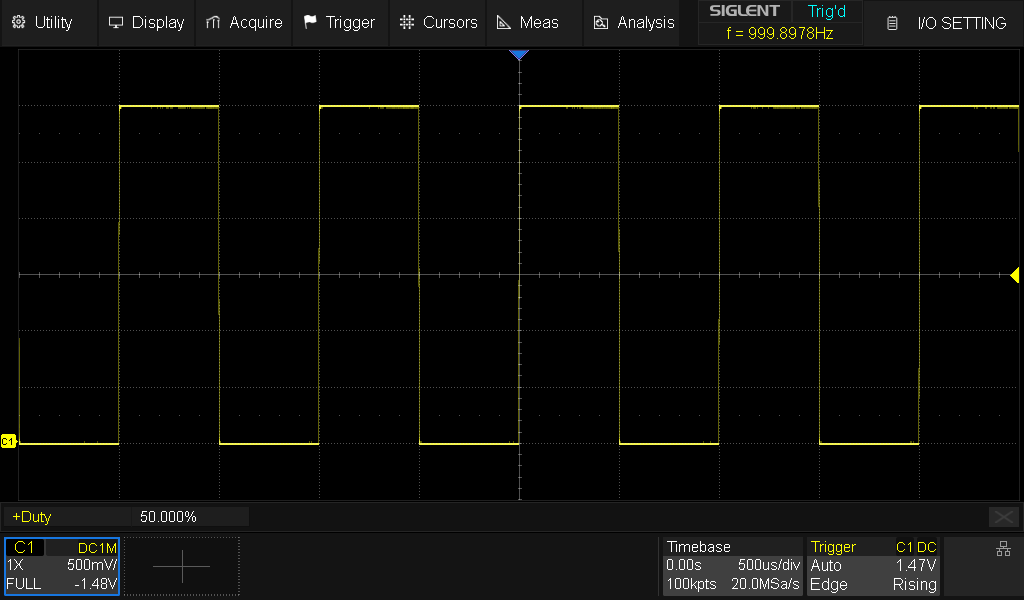
A live screen capture pulled over LAN from a Siglent SDS824X HD (its 1 kHz calibration square wave), via scope.screen_capture.get_screenshot_pil().

Features

Core Features

Programmatic API: Control your oscilloscope from Python scripts
Multi-Vendor Oscilloscope Support: Siglent (legacy SDS1000X-E/SDS2000X Plus and modern SDS800X HD/SDS5000X dialects), Tektronix, and LeCroy, auto-detected from *IDN?
Power Supply & DAQ Support: drive Siglent SPD-series power supplies and SCPI data-acquisition/data-logger units alongside the scope
Automation & Data Collection: High-level API for batch capture, continuous monitoring, and analysis
GUI Application: Modern PyQt6-based graphical interface
Waveform Acquisition: Capture and download waveform data in multiple formats (.npz, .csv, .mat, .h5)
Acquisition Provenance: every saved waveform records the instrument, settings, and timestamp that produced it; extract raw data from any saved file with load_waveform() or the scpi-extract CLI
Synthetic Signals & Realistic Mock: generate parameterized test waveforms (sine/square/triangle/ramp/DC/noise/chirp/exponential/pulse/multitone) with SignalSpec/make_waveform, or synthesize()/stream() for one-shot arrays and phase-continuous, optionally real-time-paced chunks; develop without hardware against a mock scope that synthesizes state-coupled, trigger-aligned waveforms by default
Channel Configuration: Control voltage scale, coupling, offset, bandwidth
Trigger Settings: Configure trigger modes, levels, edge detection
Advanced Analysis: Built-in FFT, SNR, THD, and statistical analysis tools

GUI Features (New!)

High-Performance Live View: Real-time waveform display (5-20 fps, configurable) using PyQtGraph
Interactive Visual Measurements: Click-and-drag measurement markers directly on waveforms
- 15+ measurement types: Frequency, Vpp, Rise Time, Duty Cycle, etc.
- Visual gates and markers with real-time calculation
- Save/load measurement configurations
- Export results to CSV/JSON
Non-Blocking Updates: Threaded data acquisition keeps GUI responsive
Reference Waveforms: Save, overlay, and compare waveforms
Protocol Decoding: I2C, SPI, UART, CAN, LIN support
Math Functions: Custom math expressions on waveforms
VNC Display: Embedded oscilloscope screen viewer

Automated Test Report Generation 📊

Automatically generate comprehensive PDF and Markdown test reports from your waveform captures with detailed analysis, visualizations, and AI-powered insights. Perfect for documentation, test validation, and automated quality control.

# Install report generator dependencies
# pip install "SCPI-Instrument-Control[report-generator]"

from datetime import datetime
from pathlib import Path

from scpi_control.report_generator.generators.markdown_generator import MarkdownReportGenerator
from scpi_control.report_generator.generators.pdf_generator import PDFReportGenerator
from scpi_control.report_generator.models.report_data import ReportMetadata, TestReport, TestSection, WaveformData

# time_data / voltage_data: your captured numpy arrays (e.g. from scope.get_waveform)
waveform = WaveformData(channel="CH1", time=time_data, voltage=voltage_data, sample_rate=1e6, record_length=len(voltage_data))

metadata = ReportMetadata(title="Probe Calibration Test Report", technician="Lab Technician", test_date=datetime.now(), equipment_model="SDS824X HD")
report = TestReport(metadata=metadata)
report.add_section(TestSection(title="Waveform Captures", waveforms=[waveform], order=1))
report.overall_result = report.calculate_overall_result()

MarkdownReportGenerator().generate(report, Path("calibration_report.md"))
PDFReportGenerator().generate(report, Path("calibration_report.pdf"))

Key Features:

✅ Automatic Signal Detection - FFT-based classification (sine, square, triangle, pulse, etc.)
✅ Comprehensive Statistics - 25+ parameters including Vpp, RMS, frequency, SNR, THD, jitter, overshoot
✅ Template Presets - Ready-made report templates such as ReportTemplate.create_probe_calibration_template(), manageable from the GUI's Template Manager
✅ Local-LLM Analysis - Optional AI insights and Q&A tool-calling via Ollama running on your own machine (no cloud providers, no API keys)
✅ Region Extraction - Zoom into plateaus, edges, and transients with calibration guidance
✅ Multiple Formats - Generate PDF and Markdown reports with embedded plots
✅ Professional Layout - Publication-ready reports with metadata, statistics tables, and visualizations
✅ Comparison & Batch Reports - Compare before/after captures or aggregate multi-DUT batches with delta/yield tables, a sign-off block, and a SHA-256 raw-data manifest; available via Report → Comparison / Batch Report… in the GUI

Report Sections Include:

Test metadata (title, ID, operator, timestamp, scope model)
Waveform plots with automatic scaling
Signal classification and characteristics
Detailed measurement tables
Region-of-interest analysis with zoomed views
AI-generated insights and recommendations (optional)
Pass/fail criteria and test conclusions

See examples/probe_calibration_analysis.py for complete examples including region extraction and automated probe compensation guidance.

Vector Graphics / XY Mode (Fun! 🎨)

Use your oscilloscope as a vector display by generating waveforms for XY mode:

Draw Shapes: Circles, rectangles, stars, polygons, Lissajous figures
Text Rendering: Display text messages on your oscilloscope screen
Animations: Create rotating and transforming graphics
Composite Paths: Combine multiple shapes into complex drawings

Requirements: External AWG/DAC or scope's built-in AWG to feed generated waveforms into scope channels.

# Install the fun extras
# pip install "SCPI-Instrument-Control[fun]"

from scpi_control import Oscilloscope
from scpi_control.vector_graphics import Shape

scope = Oscilloscope('192.168.1.100')
scope.connect()

# Enable XY mode (CH1=X, CH2=Y)
scope.vector_display.enable_xy_mode()

# Generate waveforms for a circle
circle = Shape.circle(radius=0.8, points=1000)
x_wave, y_wave = scope.vector_display.draw(circle)

# Save for AWG upload
scope.vector_display.save_waveforms(circle, "my_circle", format='csv')
# Load my_circle_x.csv and my_circle_y.csv into your AWG!

See examples/vector_graphics_xy_mode.py for more demos including animations and text!

Installation

From PyPI (recommended)

pip install SCPI-Instrument-Control

To include optional features, use extras:

# GUI application with PyQt6
pip install "SCPI-Instrument-Control[gui]"

# Automated report generation (PDF/Markdown with AI analysis)
pip install "SCPI-Instrument-Control[report-generator]"

# Vector graphics and XY mode (draw shapes on scope!)
pip install "SCPI-Instrument-Control[fun]"

# Browser-based lab gateway (scpi-web)
pip install "SCPI-Instrument-Control[web]"

# USB/GPIB/serial instruments via PyVISA
pip install "SCPI-Instrument-Control[usb]"

# Everything
pip install "SCPI-Instrument-Control[all]"

Note: The siglent-gui command includes automatic dependency checking. If you try to run the GUI without the required packages, you'll receive a clear error message with installation instructions. Missing optional dependencies (like PyQtGraph for high-performance live view) will trigger warnings but allow the GUI to launch.

Command-line tools

Command	Description
`siglent-gui`	Launch the PyQt6 GUI application
`siglent-report-generator`	Launch the standalone report-generator app
`scpi-web`	Serve the browser-based lab gateway (REST + WebSocket API, optional web UI)
`scpi-extract`	Inspect or export a saved waveform file from the command line

From source

git clone git@github.com:little-did-I-know/SCPI-Instrument-Control.git
cd SCPI-Instrument-Control
pip install -e .

Install with GUI support from source:

pip install -e ".[gui]"

Development installation

pip install -e ".[dev]"

Build & Publish (PyPI)

To create release artifacts that render correctly on PyPI:

python -m build
twine check dist/*

The twine check command validates the built distributions, including the long description rendered from README.md, before upload.

Migration Guide

v1.0.0 introduces a package rename from Siglent-Oscilloscope to SCPI-Instrument-Control to better reflect the expanded capabilities of this library.

For Existing Users

If you're upgrading from the old siglent package:

1. Update Your Installation

Uninstall the old package (if installed):

pip uninstall siglent

Install the new package:

pip install SCPI-Instrument-Control

Or with extras:

pip install "SCPI-Instrument-Control[gui]"
pip install "SCPI-Instrument-Control[all]"

2. Update Your Import Statements

Old imports (no longer work as of v2.0.0):

from siglent import Oscilloscope, PowerSupply, FunctionGenerator
from siglent.gui.app import main
from siglent.waveform import Waveform

New imports (recommended):

from scpi_control import Oscilloscope, PowerSupply, FunctionGenerator
from scpi_control.gui.app import main
from scpi_control.waveform import Waveform

3. Backward Compatibility

The siglent compatibility shim was removed in v2.0.0 (it had emitted a DeprecationWarning since v1.0.0). import siglent now raises ModuleNotFoundError — update your imports to scpi_control as shown above; the API is otherwise identical. If you cannot migrate yet, pin SCPI-Instrument-Control<2.0.

4. Command-Line Tools

The CLI commands remain unchanged for convenience:

siglent-gui                    # Still works!
siglent-report-generator       # Still works!

No changes needed to scripts or automation that invoke these commands.

5. What Changed

Old	New	Status
PyPI package: `siglent`	PyPI package: `SCPI-Instrument-Control`	Changed
`import siglent`	`import scpi_control`	Required since v2.0.0
`siglent-gui` command	`siglent-gui` command	Unchanged
`siglent-report-generator` command	`siglent-report-generator` command	Unchanged

6. Why the Rename?

This library has grown significantly beyond its original focus on Siglent oscilloscopes:

Multi-Instrument Support: Oscilloscopes, power supplies, and function generators
Multi-Vendor Support: Works with any SCPI-compatible equipment (not just Siglent)
Universal Protocol: Based on industry-standard SCPI commands

The new name better represents what the library does: control any SCPI-compatible test equipment.

Need Help?

If you encounter any migration issues:

Check the CHANGELOG.md for detailed v1.0.0 release notes
Open an issue on GitHub
Review the updated examples/ directory for new usage patterns

Quick Start

Programmatic Usage

from scpi_control import Oscilloscope

# Connect to oscilloscope
scope = Oscilloscope('192.168.1.100')
scope.connect()

# Get device information
print(scope.identify())

# Configure channel 1
scope.channel1.set_scale(1.0)  # 1V/div
scope.channel1.set_coupling('DC')
scope.channel1.enable()

# Capture waveform
waveform = scope.get_waveform(channel=1)
print(f"Captured {len(waveform.time)} samples")

scope.disconnect()

GUI Application

siglent-gui

Or from Python:

from scpi_control.gui.app import main
main()

Requirements

Core Library

Python 3.9+
NumPy >= 1.24.0
Matplotlib >= 3.7.0
SciPy >= 1.10.0

GUI Application (optional)

Install with [gui] extra to add:

PyQt6 >= 6.6.0
PyQt6-WebEngine >= 6.6.0
PyQtGraph >= 0.13.0 (high-performance plotting)

Optional Extras

Report Generator: Install with [report-generator] to add PyQt6, Pillow, requests, ReportLab, Ollama (PDF/Markdown reports with AI)
HDF5 support: Install with [hdf5] to add h5py >= 3.8.0
Vector Graphics: Install with [fun] to add shapely, Pillow, svgpathtools (XY mode drawing)
Web Gateway: Install with [web] to add FastAPI, Uvicorn, Pillow (browser-based lab gateway, scpi-web)
USB/GPIB/Serial: Install with [usb] to add PyVISA + pyvisa-py (USB-TMC, GPIB, and serial instrument connections)
All features: Install with [all] for complete functionality

Connection

The oscilloscope must be connected to your network. The default SCPI port is 5025.

To find your oscilloscope's IP address:

Press Utility on the oscilloscope
Navigate to I/O settings
Check the LAN configuration

GUI Application Overview

The SCPI Instrument Control GUI provides a comprehensive interface for controlling your oscilloscope, capturing waveforms, and performing measurements.

Main Window

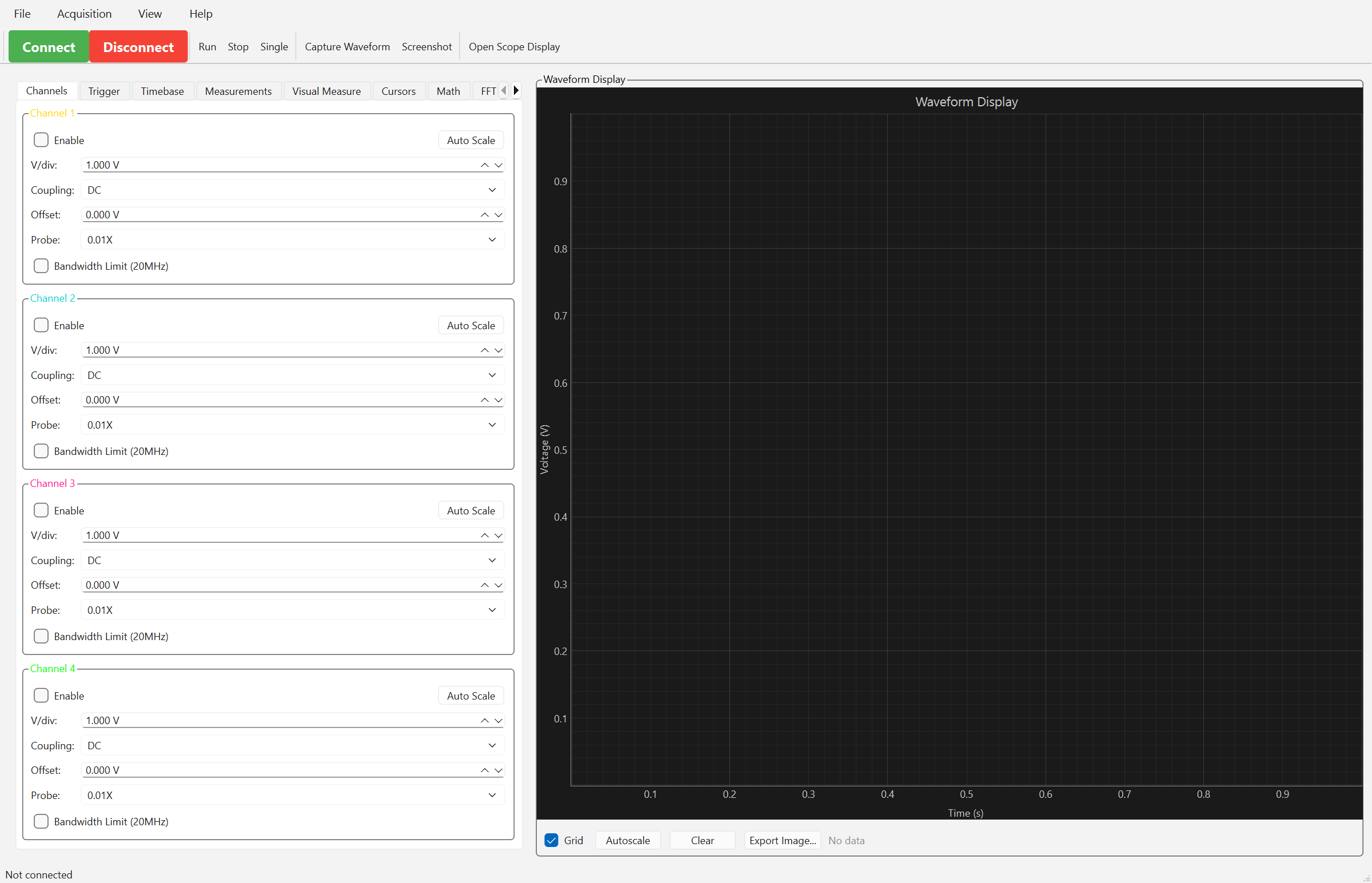
The main interface consists of:

Waveform Display: High-performance real-time plotting area (center)
Control Panels: Tabbed interface with all oscilloscope controls (right)
Menu Bar: File operations, acquisition controls, and utilities (top)
Status Bar: Connection status and system information (bottom)

Getting Connected

To connect to your oscilloscope:

Launch the GUI: siglent-gui
Enter your oscilloscope's IP address
Click Connect

The oscilloscope must be connected to your network (default SCPI port: 5025).

Finding your oscilloscope's IP address:

Press Utility on the oscilloscope
Navigate to I/O settings
Check the LAN configuration

Channel Controls

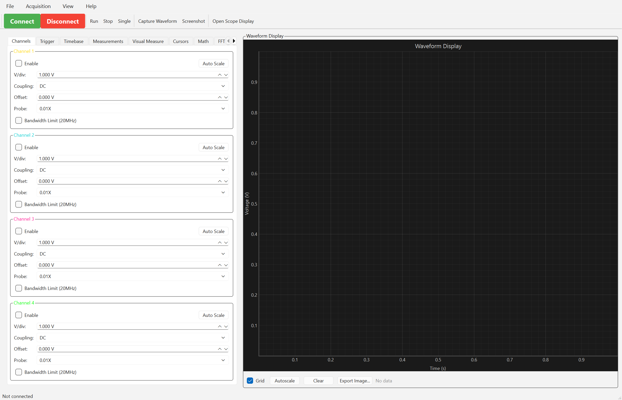
The Channels tab provides complete control over all input channels:

Enable/Disable: Toggle channels on/off with checkboxes
Voltage Scale: Adjust volts/division (0.001V to 10V)
Coupling: Set DC, AC, or GND coupling
Probe Ratio: Configure probe attenuation (1X, 10X, 100X, etc.)
Bandwidth Limit: Enable 20MHz bandwidth limiting
Offset: Adjust vertical position

Quick Tip: Enable channels before starting Live View or capturing waveforms.

GUI Application Guide

Live View

The GUI features high-performance real-time waveform viewing powered by PyQtGraph:

Acquisition → Live View (Ctrl+R)

Performance:

Real-time updates at 5-20 fps (configurable)
100x faster than traditional matplotlib-based viewers
Non-blocking: GUI remains responsive during data acquisition
Supports all 4 channels simultaneously

Controls:

Enable channels in the "Channels" tab first
Live view automatically acquires from enabled channels
Adjust update rate by modifying update_interval in live_view_worker.py

Visual Measurements

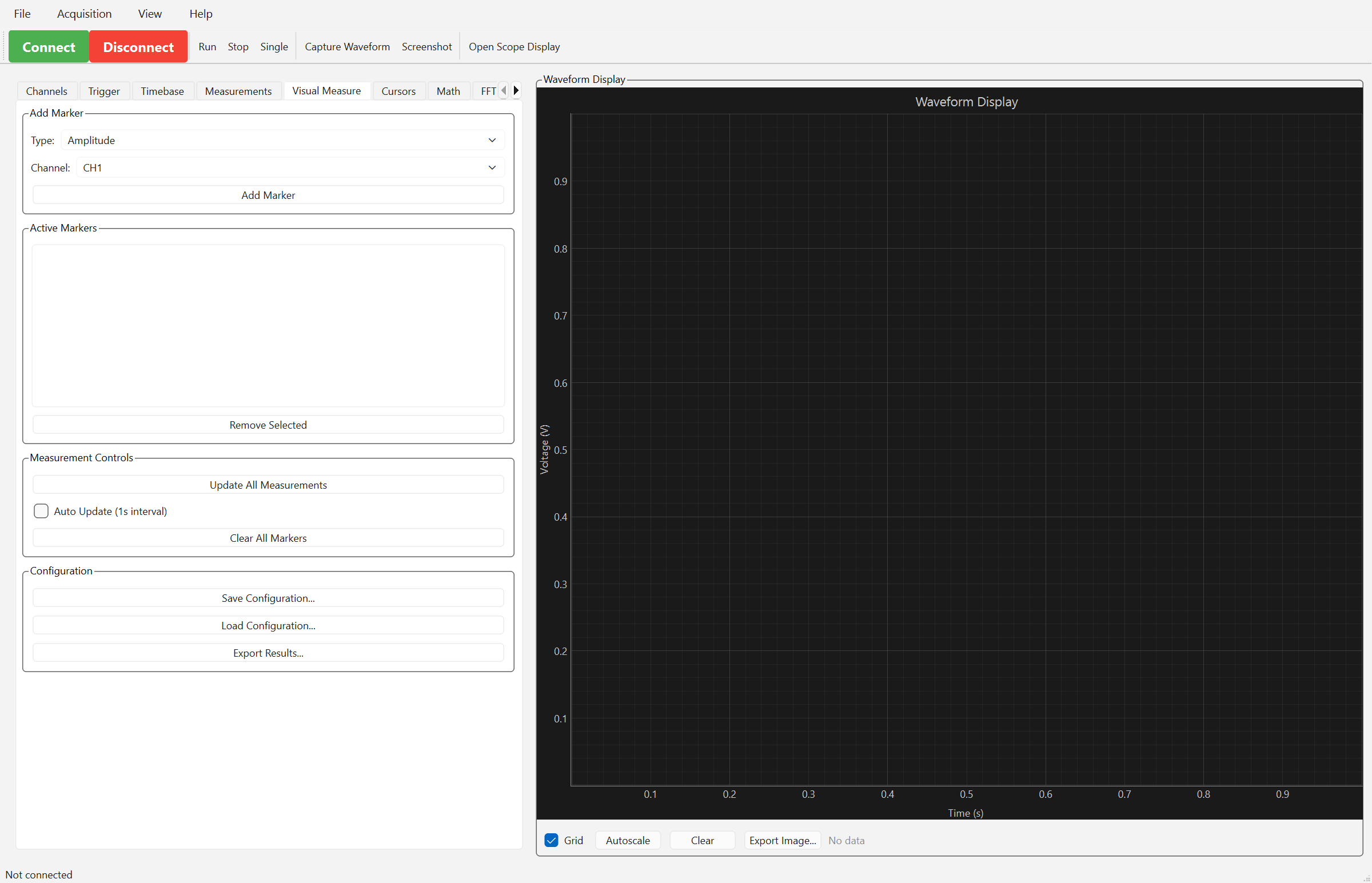
Interactive measurement markers that you can place and adjust directly on waveforms:

How to use:

Go to the "Visual Measure" tab
Select measurement type (Frequency, Vpp, Rise Time, etc.)
Select channel (CH1-CH4)
Click "Add Marker"
Marker auto-places on waveform
Drag marker gates to adjust measurement region
See real-time measurement updates

Measurement Types:

Frequency/Period: Auto-detects signal period
Voltage: Vpp, Amplitude, Max, Min, RMS, Mean
Timing: Rise Time, Fall Time, Pulse Width, Duty Cycle

Features:

Save/Load Configs: Save measurement setups for reuse
Export Results: Export to CSV or JSON
Auto-Update: Optional 1-second auto-refresh
Batch Mode: Run multiple measurements simultaneously

Example Workflow:

# In GUI:
# 1. Capture or enable live view
# 2. Visual Measure tab → Add Marker
# 3. Type: "Frequency", Channel: "CH1" → Add
# 4. Marker appears with measurement result
# 5. Save Config → "my_measurements.json"
# 6. Export Results → "results.csv"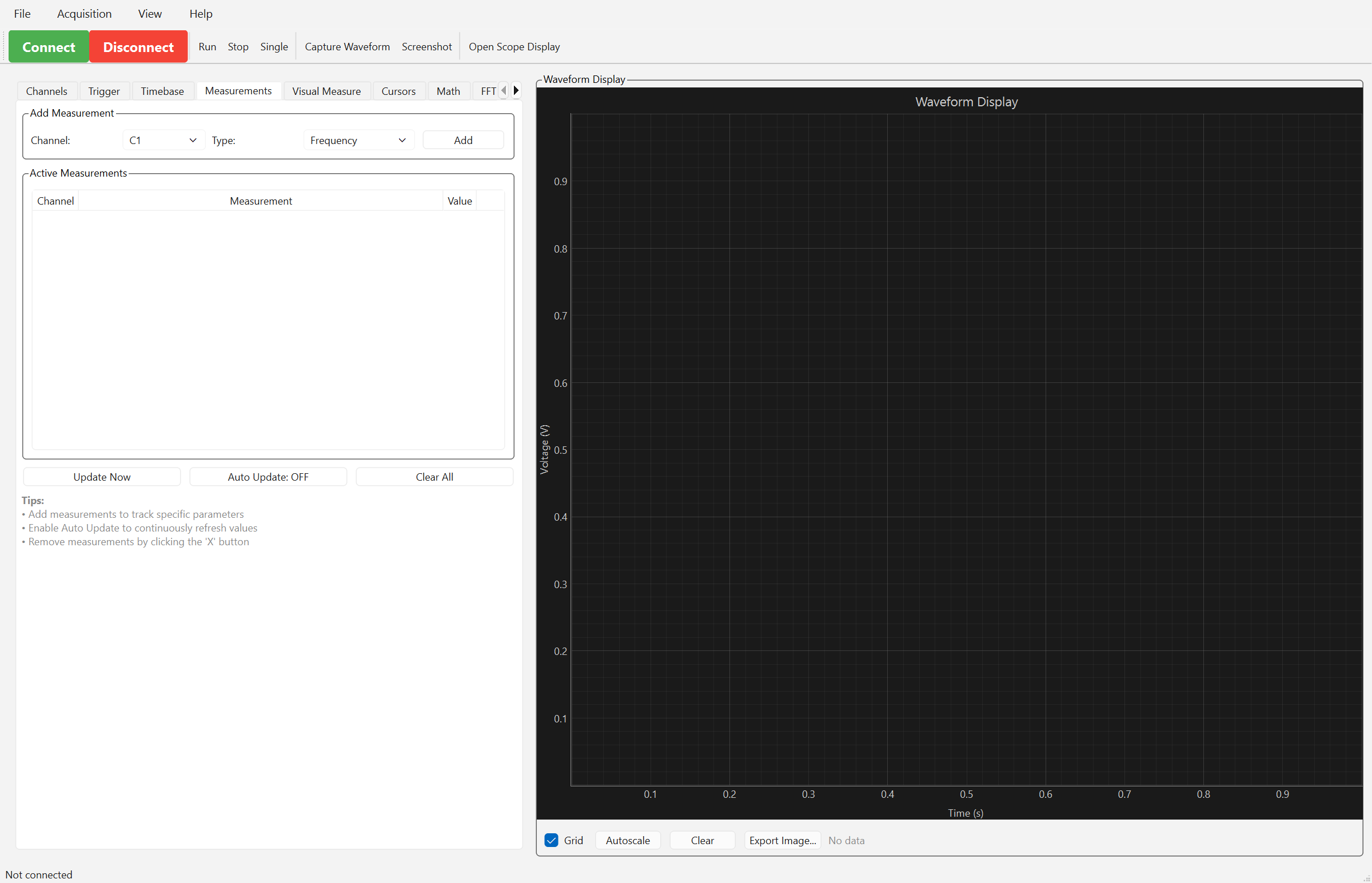

Automated Measurements

The Measurements tab provides quick access to standard oscilloscope measurements:

15+ measurement types (frequency, Vpp, RMS, rise time, etc.)
Channel selection
Results table with units
Export measurement results

Cursors

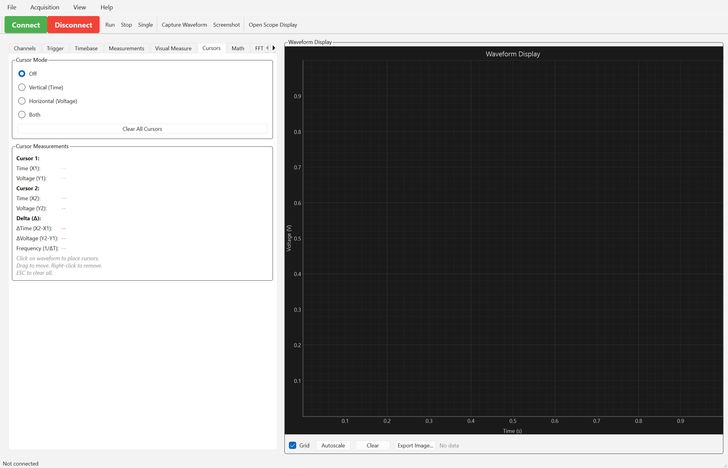
Interactive cursors for precise measurements:

Vertical cursors for time measurements
Horizontal cursors for voltage measurements
Delta calculations (ΔT, ΔV, frequency)
Draggable cursor lines
Real-time delta updates

FFT Analysis

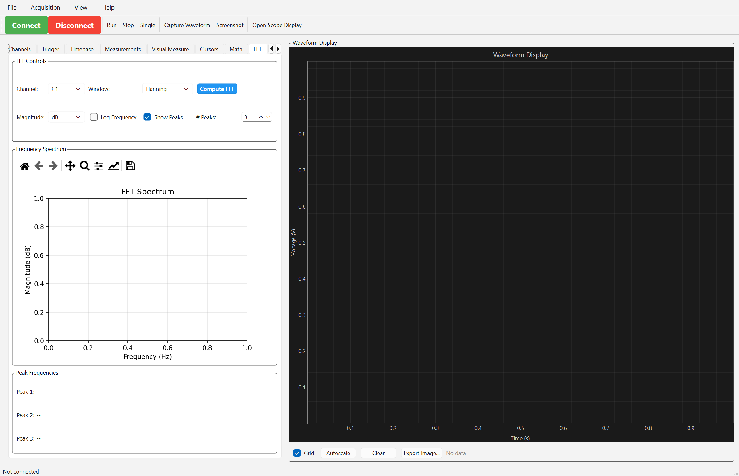
Frequency domain analysis:

Fast Fourier Transform visualization
Peak detection and markers
Window function selection (Hanning, Hamming, Blackman)
Frequency and amplitude axes
Export FFT data

Vector Graphics 🎨 (XY Mode)

Requires: pip install "SCPI-Instrument-Control[fun]"

Turn your oscilloscope into a vector display by generating waveforms for XY mode!

The Vector Graphics tab provides:

Shape Generator:

Basic Shapes: Circle, Rectangle, Star, Triangle, Line
Lissajous Figures: Classic oscilloscope patterns (3:2, 5:4, 7:5, etc.)
Parameter Controls: Adjust size, points, frequency ratios, phase shifts
Generate Button: Create vector paths with customizable parameters

Waveform Export:

Sample Rate Control: 1-1000 MSa/s for AWG compatibility
Duration: 1ms to 10s per waveform
Format Options: CSV (universal), NumPy (.npy), Binary (.bin)
Save for AWG: Exports separate X and Y waveform files

XY Mode Control:

Enable/Disable: Configure oscilloscope for XY display mode
Channel Setup: Auto-configures CH1 (X-axis) and CH2 (Y-axis)
Status Display: Connection and configuration feedback

How to use:

Go to the "Vector Graphics 🎨" tab
Select a shape (e.g., "Circle" or "Lissajous")
Adjust parameters (radius, points, frequencies)
Click "Generate Shape"
Set sample rate and duration for your AWG
Click "Save Waveforms..." to export
Load the X/Y files into your AWG (Channel 1 = X, Channel 2 = Y)
Connect AWG outputs to scope inputs
Click "Enable XY Mode" or manually enable on scope
Watch your shape appear on the oscilloscope! ✨

Works without scope connection - you can generate and export waveforms offline!

Example Use Cases:

Draw circles, stars, and geometric shapes
Create classic Lissajous patterns for calibration
Generate animations (rotating shapes, morphing patterns)
Educational demonstrations of XY mode
Signal generator pattern testing

See examples/vector_graphics_xy_mode.py for programmatic usage and animation examples.

Other GUI Features

Power Supply:

Dedicated Power Supply tab (Connect to Power Supply... menu action) for Siglent SPD-series and generic SCPI-99 power supplies
Per-channel voltage/current setpoints, output enable, and readback

Data Logger:

Dedicated Data Logger tab (Connect to Data Logger... menu action) for SCPI DAQ/data-acquisition units
Channel scan configuration and readings display

Terminal:

Built-in Terminal tab for sending raw SCPI commands directly to the connected instrument

Reference Waveforms:

Save waveforms as references
Overlay comparisons
Difference mode (live - reference)
Calculate correlation

Math Channels:

Custom expressions: C1 + C2, C1 * 2, etc.
Real-time calculation

FFT Analysis:

Frequency domain visualization
Window function selection
Peak detection

Protocol Decode:

I2C, SPI, UART, CAN, LIN decoding
Packet analysis and export

Web Gateway (beta)

Control instruments from any browser on your LAN:

pip install scpi-instrument-control[web]   # includes the browser gateway
scpi-web                                   # first run prints a URL with a token

On first run the gateway mints an access token and prints a ready-to-open URL (http://127.0.0.1:8765/?token=…). Every request needs a token — mint more with scpi-web token add <name>. Sessions can target real scopes by IP or a built-in mock (mock: true) for hardware-free use. The OpenAPI schema is served at /api/openapi.json (token required); the interactive /docs//redoc UIs are disabled. Bind to 127.0.0.1 (the default) unless your LAN is trusted, and use --host 0.0.0.0 to expose it.

Security model: the gateway authenticates every request, gives each instrument session an owner (owner writes, everyone else watches), validates outbound connection targets, and caps concurrent sessions. It does not terminate TLS — put it behind a reverse proxy or keep it on a trusted network. See the Gateway security guide for tokens, ownership, claiming, the SSRF gate, and deployment.

Upgrading from 4.x: the gateway now requires a token, and reference files saved by 4.x must be converted once with scpi-web references migrate. Both are covered in the security guide.

Full documentation: Web Gateway guide — overview, browser UI tour, and the complete REST & WebSocket API reference.

GET /api/discover scans the gateway's subnet (or ?cidr=…) for SCPI instruments on port 5025 and lists them with model and dialect — handy when DHCP moves your instruments around.
GET .../scope/screenshot.png — the instrument's display as a PNG
GET .../scope/waveform?channels=1,2&max_points=N — waveform data as JSON
GET/PATCH .../scope/math/{1,2} — software math channels (streamed as M1/M2 traces)
GET .../scope/measurements — the current measurement selection
GET/PATCH .../scope/spectrum — server-computed FFT spectrum (streamed as spectrum frames)
GET .../scope/filters + PATCH .../scope/filters/{1,2} — software Butterworth filters (streamed as F1/F2 traces)
GET/POST/DELETE .../scope/references + GET/PUT .../scope/reference — saved reference waveforms and the live overlay
POST .../scope/log/start / POST .../scope/log/stop — record the selected measurements (~1 Hz) server-side
GET .../scope/log, GET .../scope/log/data?since=, GET .../scope/log.csv — recording status, rows, and CSV export

Browser UI

make webapp-install       # once
make webapp-build         # build the UI into the server
scpi-web --host 0.0.0.0   # serve API + UI on one port

Open the tokened URL the gateway prints on startup. For UI development, run scpi-web in one terminal and cd webapp/app && npm run dev in another — Vite proxies /api (HTTP and WebSocket) to the gateway with hot reload; open the dev server with the ?token=… from the gateway's startup URL so the UI picks it up.

The home screen scans your LAN and lists instruments to connect to, resume, or open a shared session on — plus manual IP and a hardware-free mock.

API Documentation

Oscilloscope

from scpi_control import Oscilloscope

# Connect
scope = Oscilloscope('192.168.1.100', port=5025, timeout=5.0)
scope.connect()

# Device information
print(scope.identify())  # Get *IDN? string
print(scope.device_info)  # Parsed device info dict

# Basic controls
scope.run()           # Start acquisition (AUTO mode)
scope.stop()          # Stop acquisition
scope.auto_setup()    # Auto setup
scope.reset()         # Reset to defaults

Channels

# Channel configuration (channels 1-4)
scope.channel1.enable()
scope.channel1.coupling = "DC"  # DC, AC, or GND
scope.channel1.voltage_scale = 1.0  # Volts/division
scope.channel1.voltage_offset = 0.0  # Volts
scope.channel1.probe_ratio = 10.0  # 10X probe
scope.channel1.bandwidth_limit = "OFF"  # ON or OFF

# Get configuration
config = scope.channel1.get_configuration()

Trigger

# Trigger configuration
scope.trigger.mode = "NORMAL"  # AUTO, NORM, SINGLE, STOP
scope.trigger.source = "C1"  # C1, C2, C3, C4, EX, LINE
scope.trigger.level = 0.0  # Trigger level in volts
scope.trigger.slope = "POS"  # POS (rising) or NEG (falling)

# Edge trigger setup
scope.trigger.set_edge_trigger(source="C1", slope="POS")

# Trigger actions
scope.trigger.single()  # Single trigger
scope.trigger.force()   # Force trigger

Waveform Acquisition

# Acquire waveform
waveform = scope.get_waveform(channel=1)

# Access data
print(waveform.time)      # Time array (numpy)
print(waveform.voltage)   # Voltage array (numpy)
print(waveform.sample_rate)
print(waveform.record_length)

# Save waveform
scope.waveform.save_waveform(waveform, "data.csv", format="CSV")

Measurements

# Individual measurements
freq = scope.measurement.measure_frequency(1)
vpp = scope.measurement.measure_vpp(1)
vrms = scope.measurement.measure_rms(1)
period = scope.measurement.measure_period(1)

# All measurements at once
measurements = scope.measurement.measure_all(1)

Programmatic Data Collection & Automation

For advanced data collection workflows, use the high-level automation API:

from scpi_control.automation import DataCollector

# Simple capture with automatic analysis
with DataCollector('192.168.1.100') as collector:
    # Capture waveforms
    data = collector.capture_single([1, 2])

    # Analyze waveform
    stats = collector.analyze_waveform(data[1])
    print(f"Vpp: {stats['vpp']:.3f}V, Freq: {stats['frequency']/1e3:.2f}kHz")

    # Save to file - format is auto-detected from the extension (.npz/.csv/.mat/.h5)
    collector.save_data(data, 'measurement.npz')

Batch capture with configuration sweeps:

# Capture with different timebase and voltage settings
results = collector.batch_capture(
    channels=[1],
    timebase_scales=['1us', '10us', '100us'],
    voltage_scales={1: ['500mV', '1V', '2V']},
    triggers_per_config=5
)
collector.save_batch(results, 'batch_output')

Continuous time-series collection:

# Collect data over time with automated file saving
collector.start_continuous_capture(
    channels=[1, 2],
    duration=300,          # 5 minutes
    interval=1.0,          # 1 capture per second
    output_dir='time_series_data',
    file_format='npz'
)

Event-based trigger capture:

from scpi_control.automation import TriggerWaitCollector

with TriggerWaitCollector('192.168.1.100') as tc:
    # Configure trigger
    tc.collector.scope.trigger.set_source(1)
    tc.collector.scope.trigger.set_slope('POS')
    tc.collector.scope.trigger.set_level(1, 1.0)

    # Wait for trigger event
    data = tc.wait_for_trigger(channels=[1, 2], max_wait=30.0)

Advanced analysis:

# Built-in analysis includes: Vpp, RMS, frequency, SNR, THD, etc.
analysis = collector.analyze_waveform(waveform)
print(f"SNR: {analysis['snr_db']:.2f} dB")
print(f"THD: {analysis['thd_percent']:.2f}%")

See examples/ directory for complete automation examples including:

Simple capture (simple_capture.py)
Batch processing (batch_capture.py)
Continuous monitoring (continuous_capture.py)
Trigger-based capture (trigger_based_capture.py)
Advanced analysis with visualization (advanced_analysis.py)

Reading Saved Waveforms Back (`load_waveform` / `scpi-extract`)

Any file saved by the library (.npz/.csv/.mat/.h5) can be read back with load_waveform(), which normalizes format differences and reattaches acquisition provenance when present:

from scpi_control.waveform_io import load_waveform

loaded = load_waveform("measurement.npz")
print(loaded.time, loaded.voltage)          # numpy arrays
print(loaded.provenance)                    # instrument/settings snapshot, or None
df = loaded.to_dataframe()                  # pandas DataFrame, provenance in df.attrs

The same data is available from the command line via scpi-extract:

scpi-extract measurement.npz --info          # provenance + metadata summary
scpi-extract measurement.npz --csv out.csv   # dump raw time,voltage rows
scpi-extract measurement.npz --json          # machine-readable metadata

Examples

This project ships 27 runnable example scripts, each documented with its requirements in examples/README.md — see it for the full list. A few highlights:

basic_usage.py - Connection and basic operations
waveform_capture.py - Capture and save waveforms
measurements.py - Automated measurements
live_plot.py - Real-time plotting
probe_calibration_analysis.py - Automated report generation with region extraction and AI analysis
synthetic_signals.py - Generating parameterized test waveforms and streaming state-coupled mock captures (no hardware)
waveform_provenance_and_extract.py - Capturing with provenance, saving, and reading back with load_waveform() (no hardware)

Supported Models

Siglent (Fully Tested)

SDS800X HD Series: SDS804X HD, SDS824X HD
SDS1000X-E Series: SDS1102X-E, SDS1104X-E, SDS1202X-E, SDS1204X-E
SDS2000X Plus Series: SDS2104X+, SDS2204X+, SDS2354X+
SDS5000X Series: SDS5034X, SDS5054X, SDS5104X

Tektronix and LeCroy (core control + measurements)

Tektronix TBS1000C Series: TBS1102C
Tektronix 2 Series MSO: MSO24
Tektronix 4 Series MSO: MSO44, MSO46
Tektronix 5 Series MSO: MSO54, MSO56, MSO58, MSO58LP
Tektronix 6 Series MSO: MSO64
LeCroy WaveSurfer 3000z Series: WaveSurfer 3024z
LeCroy WaveRunner 8000 Series: WaveRunner 8104

All Tektronix MSO models (2/4/5/6 Series) share one command variant and support automated measurements — see the SCPI Dialects guide for the full per-vendor gap list.

Command tables were verified command-by-command against the vendor programmer manuals (Tektronix TBS1000C, 2 Series MSO, and 4/5/6 Series MSO/6 Series LPD manuals; the Teledyne LeCroy MAUI Remote Control and Automation Manual) and exercised against a dialect-aware mock; not yet run against real Tektronix or LeCroy hardware.

Function Generators

Siglent SDG1000X Series: SDG1032X, SDG1025, SDG1020
Siglent SDG2000X Series: SDG2122X, SDG2082X, SDG2042X

Power Supplies

Siglent SPD3303X Series: SPD3303X, SPD3303X-E (triple output)
Siglent SPD1000X Series: SPD1305X, SPD1168X (single output)

Data Acquisition (DAQ)

Keysight/Agilent 34970A Series: 34970A, 34972A
Keysight DAQ970A Series: DAQ970A, DAQ973A
Generic SCPI-99 data loggers via the DAQ capability registry

Compatibility

Should work with other Siglent oscilloscopes that support SCPI commands over Ethernet. Model-specific features are auto-detected via the ModelCapability registry. Unrecognized Tektronix or LeCroy models fall back to a conservative generic profile for that vendor (with a logged warning) rather than being rejected outright.

Note: Some SCPI commands vary between models. The library includes model-specific command variants for HD, X, and Plus series (Siglent) and for TBS vs. MSO (2/4/5/6 Series share one variant) (Tektronix).

Contributing

Contributions are welcome! Please read our Contributing Guide for details on:

Development setup and workflow
Code style and testing requirements
Pull request process
How to report bugs and request features

Quick Start for Contributors

# Clone and setup
git clone https://github.com/little-did-I-know/SCPI-Instrument-Control.git
cd SCPI-Instrument-Control

# Install development environment
make dev-setup

# Run tests
make test

# Format code
make format

# Run all checks
make check

During development, python -m pytest --testmon runs only the tests affected by your changes for fast feedback; the full suite is still required before opening a PR.

See our Code of Conduct and Security Policy for more information.

Community and Support

Issues: Report bugs or request features
Discussions: Ask questions and share ideas
Security: See our Security Policy for reporting vulnerabilities

Resources

📘 Interactive Tutorial - Jupyter notebook with step-by-step examples
📁 Examples Directory - Ready-to-run example scripts
📖 API Documentation - Complete API reference in this README
🔧 Contributing Guide - How to contribute to the project
🧪 Experimental Features Guide - Beta releases and experimental features
🔒 Security Policy - Security best practices and reporting

License

MIT License - see LICENSE file for details

Name		Name	Last commit message	Last commit date
Latest commit History 764 Commits
.github		.github
docs		docs
example_reports		example_reports
examples		examples
resources		resources
scpi_control		scpi_control
scripts		scripts
tests		tests
webapp		webapp
.codecov.yml		.codecov.yml
.docstring-validation.yaml		.docstring-validation.yaml
.editorconfig		.editorconfig
.gitignore		.gitignore
.pre-commit-config.yaml		.pre-commit-config.yaml
.readthedocs.yml		.readthedocs.yml
BRANDING.md		BRANDING.md
BUILD_EXECUTABLE.md		BUILD_EXECUTABLE.md
CHANGELOG.md		CHANGELOG.md
CONTRIBUTING.md		CONTRIBUTING.md
LICENSE		LICENSE
MANIFEST.in		MANIFEST.in
Makefile		Makefile
README.md		README.md
REPORT_GENERATOR_FEATURE.md		REPORT_GENERATOR_FEATURE.md
SECURITY.md		SECURITY.md
mkdocs.yml		mkdocs.yml
pyproject.toml		pyproject.toml
report-generator-linux.spec		report-generator-linux.spec
report-generator-windows.spec		report-generator-windows.spec
siglent-gui.spec		siglent-gui.spec
test_report.pdf		test_report.pdf

Folders and files

Latest commit

History

Repository files navigation

SCPI Instrument Control

Features

Core Features

GUI Features (New!)

Automated Test Report Generation 📊

Vector Graphics / XY Mode (Fun! 🎨)

Installation

From PyPI (recommended)

Command-line tools

From source

Development installation

Build & Publish (PyPI)

Migration Guide

For Existing Users

1. Update Your Installation

2. Update Your Import Statements

3. Backward Compatibility

4. Command-Line Tools

5. What Changed

6. Why the Rename?

Need Help?

Quick Start

Programmatic Usage

GUI Application

Requirements

Core Library

GUI Application (optional)

Optional Extras

Connection

GUI Application Overview

Main Window

Getting Connected

Channel Controls

GUI Application Guide

Live View

Visual Measurements

Automated Measurements

Cursors

FFT Analysis

Vector Graphics 🎨 (XY Mode)

Other GUI Features

Web Gateway (beta)

Browser UI

API Documentation

Oscilloscope

Channels

Trigger

Waveform Acquisition

Measurements

Programmatic Data Collection & Automation

Reading Saved Waveforms Back (load_waveform / scpi-extract)

Examples

Supported Models

Siglent (Fully Tested)

Tektronix and LeCroy (core control + measurements)

Function Generators

Power Supplies

Data Acquisition (DAQ)

Compatibility

Contributing

Quick Start for Contributors

Community and Support

Resources

License

About

Topics

Resources

Contributing

Security policy

Stars

Watchers

Forks

Releases

Packages

Contributors

Languages

Reading Saved Waveforms Back (`load_waveform` / `scpi-extract`)